Confirmatory Factor Analysis and Measurement Invariance

Factor Analysis

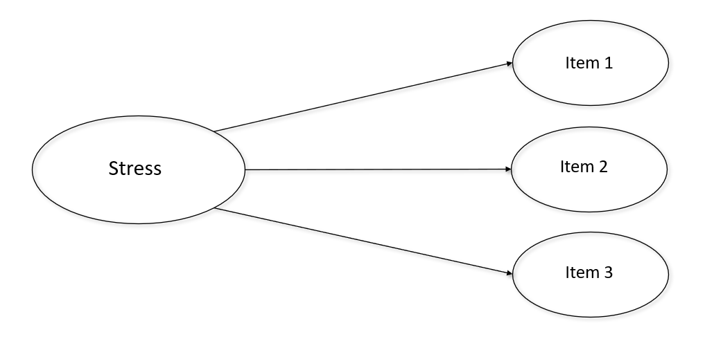
Many constructs of interest related to human behavior, attitude, identity, and motivation are not directly observable. For example, the Depression, Anxiety, and Stress scale (DASS) measures individuals’ perceptions of their depression, anxiety, and stress. We can not directly measure any of these constructs, so we refer to them as “latent variables”. We have to infer a latent variable’s value using other means. One common way to do this is by asking individuals a number of questions on a survey that we assume are predicted by the latent construct of interest (e.g. stress, Figure 1).

Another useful feature of latent variables is they allow us to reduce the number of items used in future analyses by combining a number of similar items into one variable. To validate a latent variable, and make sure the items we choose are accurately representing it, we need to confirm two assumptions:

1. We need to be sure the items which are supposedly predicted by the latent variable actually are.

AND

2. We need to ensure that the survey items we choose function similarly across different groups of individuals in the sample. That is, the items need to be invariant between groups.

In order to confirm those two conditions are met statisticians developed an useful tool called Confirmatory Factor Analysis (CFA). Testing measurement invariance is simply using CFA to test differences between groups (e.g. ethnicity) in a sample. Note that there is also something called Principle Components Analysis (PCA), which is slightly different from CFA; however, we will not discuss that difference here. For practical application purposes CFA will suffice.

In this analysis I will examine how depression, anxiety, and stress survey items load on to a number of different factors. Although with this data we can assume there are three latent variables, oftentimes researchers will not be sure how many latent factors there really. For demonstration’s sake we will assume that the number of latent variables in this dataset is unclear. If that is the case, the first order of business is to conduct an exploratory factor analysis (EFA) which we can use to establish the number of factors present in the data. Once we establish the number of factors, we can confirm the factor structure with a CFA. Importantly, it is unwise to run an EFA and CFA with the same data, so randomly splitting the dataset into two equal halves is the first step here.

# Setting seed to reproduce example and reducing sample size so analyses run faster.
set.seed(101)
sample_df <- sample_n(sample_df, 5000)

#Splitting dataset in half. 
v <- as.vector(c(rep(TRUE,2500),rep(FALSE,2500)))
ind <- sample(v)
efa_df <- sample_df[ind, ] 
cfa_df <- sample_df[!ind, ] 

After loading the ‘psych’ package, let’s do a parallel analysis to get an idea of how many factors might be in our data. In a parallel analysis we can use an eigenvalue of >1 and the FA simulated and resampled data to guide us selecting the appropriate number of factors.

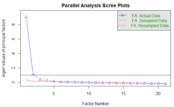
We can see that the ideal factor structure appears to be somewhere between 2 and 4 factors, since 2 is how many factors have an eigenvalue of greater than 1, and 4 is about how many factor are above the simulated/resamples lines. So, let’s we will run an EFA using 2, 3, and 4 factors.

efa_fit <- fa(efa_df, nfactors = 2, rotate = "oblimin", fm = "ml")
print(efa_fit, cut = 0.3)
efa_fit$loadings
fa.diagram(efa_fit)

efa_fit2 <- fa(efa_df, nfactors = 3, rotate = "oblimin", fm = "ml")
print(efa_fit2, cut = 0.3)
efa_fit2$loadings
fa.diagram(efa_fit2)

efa_fit2 <- fa(efa_df, nfactors = 4, rotate = "oblimin", fm = "ml")
print(efa_fit2, cut = 0.3)
efa_fit2$loadings
fa.diagram(efa_fit2)

After running the above code we can conclude that there are most likely 3 factors in this data, consistent with our theoretical understanding of the survey items. Next, we will use the other half of our sample to conduct a CFA to confirm that the 3 factor solution does indeed describe the data well. We will specify the variables in our CFA as they are theoretically described in the survey:

model.dass <-'
    stress =~ Q22A + Q6A + Q12A + Q39A + Q8A + Q14A + Q18A
    anxiety =~ Q2A + Q4A + Q41A + Q40A + Q28A + Q19A + Q20A
    depression =~ Q3A + Q42A + Q10A + Q26A + Q31A + Q17A + Q38A 
    '

After specifying the model we then check to see how well the model fits the data:

fit.dass <- cfa(model.dass, data = cfa_df, missing = "fiml", estimator = "ML")
summary(fit.dass, fit.measures = TRUE, standardized = TRUE)

Notice that “fiml” is used to deal with missing data. Fiml is generally quite robust to non-MCAR data and is a good choice most of the time. I also use the “ML” estimator , which is a good choice for most analyses (if you have multilevel data you will want to use the MLR estimator to adjust for robust SE). In the summary function we choose to include fit statistics and standardized versions of the estimates.

After running the code above we see a long output that gives us a variety of information, but only the pertinent fit information is included below:

User Model versus Baseline Model:

  Comparative Fit Index (CFI)                    0.949
  Tucker-Lewis Index (TLI)                       0.943

Loglikelihood and Information Criteria:

  Loglikelihood user model (H0)             -65949.025
  Loglikelihood unrestricted model (H1)     -65187.621
                                                      
  Akaike (AIC)                              132030.049
  Bayesian (BIC)                            132414.437
  Sample-size adjusted Bayesian (BIC)       132204.738

Root Mean Square Error of Approximation:

  RMSEA                                          0.054
  90 Percent confidence interval - lower         0.051
  90 Percent confidence interval - upper         0.056
  P-value RMSEA <= 0.05                          0.008

Standardized Root Mean Square Residual:

  SRMR                                           0.032

Important indicators of a good fitting model include:

1. CFA/TLI > 0.9 (ideally above 0.95)
2. RMSEA/SRMR < 0.8 (ideally less than 0.5)
3. Standardized loadings > 0.5

We can see that the model fit is acceptable (standardized loadings are not show, but all are above 0.5). Now that we know the model fits well and all items load on to their appropriate factors with standardized loadings greater than 0.5 we need to see if this factor structure functions the same across all groups of interest. In this study we are interested in determining if these measures function similarly between people who vote and those who do not vote. To do this we model some multi-group CFAs to test for measurement invariance.

Measurement Invariance

It is possible to achieve four levels of measurement invariance, with each successive level representing increasingly constrained models across groups. The higher the level of invariance achieved, the more similar the various groups perceive the meanings of the items to be. The levels of invariance from least to most constrained are:

1. Configural
2. Weak
3. Strong
4. Strict

The level of invariance required depends on what subsequent analysis we have planned. Notably, strict invariance is not a necessary requirement for most analyses. The lavaan package makes modeling multi-group CFAs very simple. To specify the configural model we use the same CFA model as before, we just add the “group” argument to the CFA function and specify the variable which indicates the our groups:

#Recoding 0 to NA in the voted variable.
cfa_df$voted <- replace(cfa_df$voted, cfa_df$voted == 0, NA)


#Configural invariant MI model.
model.mi <- ' 
    stress =~ Q22A + Q6A + Q12A + Q39A + Q8A + Q14A + Q18A
    anxiety =~ Q2A + Q4A + Q41A + Q40A + Q28A + Q19A + Q20A
    depression =~ Q3A + Q42A + Q10A + Q26A + Q31A + Q17A + Q38A 
'
fit.config <- cfa(model.mi, data = cfa_df, missing = "fiml", group = "voted",  estimator = "ML")
summary(fit.config, fit.measures = TRUE, standardized = TRUE)

The configural model ends up fitting well, so we then check weak invariance. Weak invariance imposes restraints on factor loadings, constraining them to be equal across groups. Since the same model is used for each level of invariance, lavaan lets us add an argument to specify that factor loadings should be equal between groups:

fit.weak <- cfa(model.mi, data = cfa_df, missing = "fiml", group = "voted", group.equal = "loadings",  estimator = "ML")
summary(fit.weak, fit.measures = TRUE, standardized = TRUE)

To see if weak invariance is achieved we need to compare the fit between the configural and weak models. If the weak model does not fit significantly worse than the the configural model, then we can retain the weak invariance hypothesis. To test difference in model fit we can either use a chi square difference test, or evaluate the difference in the CFI test statistic. A general rule of thumb states that if the change in CFI between models is <= 0.01 we can accept the more constrained model. Since the chi square test is susceptible to sample size issues, especially as observations climb above 200 – 300, we will use the difference in CFI here.

Configural model CFI = 0.948

Weak model CFI = 0.947

0.948 – 0.947 = 0.001

Therefore, we conclude we have achieved weak invariance. Now, we repeat the same process to test for strong and strict invariance. Strong invariance assumes the intercepts of all items are equal across groups, and strict invariance constrains the variances of residuals to be equal across groups.

fit.strong <- cfa(model.mi, data = cfa_df, missing = "fiml", group = "voted", group.equal = c("loadings", "intercepts"),  estimator = "ML")
summary(fit.strong, fit.measures = TRUE, standardized = TRUE)

fit.strict <- cfa(model.mi, data = cfa_df, missing = "fiml", group = "voted", group.equal = c("loadings", "intercepts", "residuals"),  estimator = "ML")
summary(fit.strict, fit.measures = TRUE, standardized = TRUE)

In the end, we achieve strict measurement invariance between groups of voters and non-voters. Therefore, we are free to proceed with further analyses, confident in the fact that the structure of our latent variables is robust between these groups. We can repeat this process with as many other grouping variables that are of interest to us.

What happens if your CFA or measurement invariance models do NOT fit well? THAT is a story for another post!

***Check out the Github repository for this post to access the data and R script***