Multilevel data are those data which are ordered in a hierarchy, data that has a “nested” structure. A common nesting structure is having multiple measurements within one subject. For example, if we measure students’ engagement in science class several times over the course of an entire semester the data we get has a specific hierarchy. We have multiple observations per student, and multiple students in each classroom.
Since this nesting structure exists, we can no longer assume that each observation is independent of one another (it is likely that observations within a single person and even within the same classroom are related in some way), thus violating a key assumption of OLS regression (and many other statistical models). Although this will not bias the coefficient estimates, it WILL underestimate SEs. The underestimation of SEs can lead to increased Type II errors (falsely concluding there is no significant effect when there actually is), and no one wants that! One common way to tackle this issue is by using multilevel models; however, sometimes we may only want to get a sense of correlations in multilevel data, instead of running an entire multilevel model, before we move on to a different type of analysis (e.g. mixture models). What to do?
Enter within-subject correlations. Modeling correlations without taking into account the nesting structure of the observations may hid important intra-individual associations. Luckily, there is a handy R package, rmcorr, that allows us to calculate within-subject correlations.
For this example I will use a dataset built into the rmcorr package, bland1995. This dataset contains data on 8 individuals’ pH and PacO2 levels. First, I’ll save the dataset and give the variables and values some labels (not necessary, but nice to do):
library(rmcorr)
library(tidyverse)
library(labelled)
library(Hmisc)

bland <- bland1995

#Labeling variables and values
var_label(bland) <- c(Subject = "Subject ID", pH = "Stomach pH", PacO2 = "Blood PacO2")

val_labels(bland$Subject) <- c("Subject 1" = 1, "Subject 2" = 2, "Subject 3" = 3, "Subject 4" = 4, "Subject 5" = 5, "Subject 6" = 6, "Subject 7" = 7, "Subject 8" = 8)
Now, we can use the rmcorr package to calculate the within-subject correlation between pH and PacO2:
bland$Subject <- as.factor(bland$Subject)
bland.rmcorr <- rmcorr(participant = Subject, pH, PacO2, dataset = bland)
print(bland.rmcorr)

Repeated measures correlation
r
: -0.5067697

degrees of freedom: 38

p-value
: 0.0008471081

95% confidence interval
: -0.7112297 -0.223255
Great! We can see that there is a significant negative correlation between the levels of ph and PacO2. The rmcorr package also comes with a handy function that allows us to visualize the association between variables at the within-subject level:
plot(bland.rmcorr, xlab = "pH", ylab = "PacO2")
In the graph above each color represents 1 individual, so we can see that within an individual person as pH rises, PacO2 decreases, agreeing with the negative correlation we calculated previously. Ok, but now let’s take a look at what we would find if we did not take into account the multilevel nature of our data and instead calculated a correlation like we normally would (between-subjects correlation). There are a few ways to calculate a correlation with multilevel data without accounting for the nesting of observations
- Assume each observation is independent and calculate a correlation like you normally would for non-hierarchical data.
- Calculate an average value for pH and PacO2 for each subject and use those average values to calculate a correlation.
- Calculate a correlation at each time point separately and treat those values as cross-sectional
Each of these methods might be useful, depending on what your research questions are and what type of correlations you are interested in, but none accurately represent the intra-individual associations between the two variables, which is why we calculated within-subject correlations earlier. Below is code demonstrating between-subject correlations calculated assuming all observations are independent, and using the mean value of each subject for pH and PacO2:
#Calculate the correlation between pH and PacO2 treating all observations as independent
bt.corr2 <- select(bland, pH, PacO2)
rcorr(as.matrix(bt.corr2), type = "pearson")

         pH PacO2
pH     1.00 -0.07
PacO2 -0.07  1.00
n= 47

P-value
      pH     PacO2
pH           0.6632
PacO2 0.6632
#Make a dataset that contains only 1 observation from each individual while keeping all variables
df1 <- distinct(bland, Subject, .keep_all = T)
#Calculate mean values for pH and PacO2 for each subject
df2 <- bland %>%
group_by(Subject) %>%
summarise(pH_mean = mean(pH), PacO2_mean = mean(PacO2))
#Add the mean values to our dataset with 1 observation per subject
bt.corr <- left_join(df1, df2, by = "Subject")
#Calculate the correlation between means of pH and PacO2
bt.corr <- select(bt.corr, pH_mean, PacO2_mean)
rcorr(as.matrix(bt.corr), type = "pearson")
pH_mean PacO2_mean
pH_mean 1.00 0.08
PacO2_mean 0.08 1.00
n= 8
P-value
pH_mean PacO2_mean
pH_mean 0.8474
PacO2_mean 0.8474 The correlation between pH and PacO2 is not significant and is close to 0 in both calculations, much different from the within-subject correlation we calculated earlier. If we plot a graph with a regression line using the full dataset we see that the line has a slope close to 0, a stark contrast to the within-subjects graph we plotted earlier.
ggplot(bt.corr, aes(x = pH_mean, y = PacO2_mean)) +
  geom_point() +
  geom_smooth(method = lm) +
  labs(x = "pH", y = "PacO2")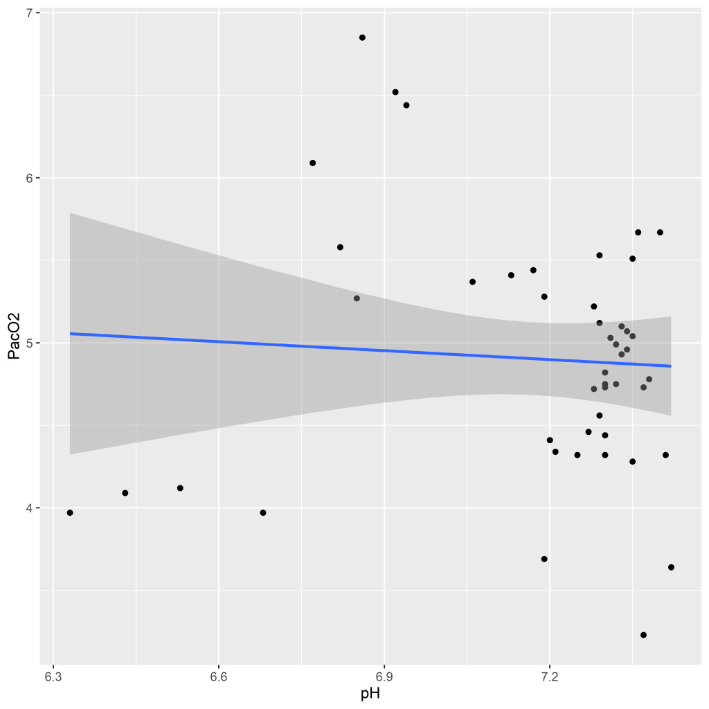
What have we learned? If we had not taken the time to calculate within-subject correlations and instead run a simple OLS regression or between-subjects correlation we would have missed an important association between pH and PacO2. Namely, that although there is no relationship between pH and PacO2 at the subject level, at the within-person level PacO2 decreases with increasing pH. Depending on the type of research and variables involved this could have substantial implications for conclusions and recommendations. So, when analyzing multilevel data, always try to account for the nested structure of your data!
***Check out the Github repository for this post to access the data and R script***
