Confirmatory Factor Analysis
In a previous post I did an exploratory and confirmation factor analysis, and measurement invariance work with data generated from the depression, anxiety, and stress scale (DASS). In that post there were no fit issues with the CFA or the measurement invariance models. However, this is often not the case when we use messy, real world data. Modifying our model to reach acceptable fit is common practice.
A word of caution though. There are statistical means to identify problem parameters and recommend methods to improve model fit; HOWEVER, be sure changes made to a model are theoretically sound. If they are not, you will just be overfitting the model to you data, and your results will still be uninterpretable. Alternatively, sometimes the model might not quite reach rule of thumb threshold fit values, but the suggested model changes do not make sense theoretically. In these cases it is almost always better to stick with theory rather than changing loadings or adding covariances that do not make sense.
Alright, let’s first take a look at our CFA model. If you need a refresher on factor analysis or measurement invariance, take a look at my previous post. You might notice we are using the same dataset (DASS survey data) from my previous post, I have just moved a couple of items around to demonstrate a poor fitting model.
library(lavaan)
library(tidyverse)
library(psych)

sample_df <- read_csv("C:/Users/schel/My Drive/Personal/Blog/CFA and MI Deeper Dive/cfa_mi_deeper_drive_data.csv")

#Reducing sample size so analyses run faster
set.seed(101)
sample_df <- sample_n(sample_df, 5000)
model.dass <-'
stmodel.dass <-'
stress =~ Q22A + Q6A + Q12A + Q39A + Q8A + Q18A
anxiety =~ Q2A + Q4A + Q41A + Q40A + Q28A + Q19A + Q20A + Q38A
depression =~ Q3A + Q42A + Q10A + Q26A + Q31A + Q17A + Q14A
'
fit.dass <- cfa(model.dass, data = sample_df, missing = "fiml", estimator = "ML")
summary(fit.dass, fit.measures = TRUE, standardized = TRUE)
Comparative Fit Index (CFI) 0.895
Tucker-Lewis Index (TLI) 0.881
RMSEA 0.078
90 Percent confidence interval - lower 0.076
90 Percent confidence interval - upper 0.080
P-value RMSEA <= 0.05 0.000
SRMR 0.0566As a reminder the commonly accepted thresholds for an good fitting SEM model are:
- CFA/TLI > 0.9 (ideally above 0.95)
- RMSEA/SRMR < 0.8 (ideally less than 0.5)
- Standardized loadings > 0.5
You’ll notice that the fit statistics are not TOO bad, but the CFI and TLI could definitely be improved. Luckily lavaan has some useful functions to help us identify potential problems with our model (remember, always make sure your changes make sense theoretically).
mod.ind <- modificationindices(fit.dass, sort = T)
View(mod.ind)
Modification indices quantitatively identify parameter changes to your model that would improve model fit. Larger modification indices indicate a larger positive impact on model fit. In the table above “lhs” stands for “left hand statement”, “op” is the lavaan operator, “rhs” is “right hand statement”, and “mi” is modification index. So, we can see that loading Q38A onto the depression factor is the most “bang for our buck” so to speak, meaning, this change would improve model fit the most out of any other change we could make. Its best practice to make one change at a time, and recheck mod indices after each change to your model. After thinking about whether loading Q38A on to the depression factor instead of the anxiety factor makes theoretical sense, let’s go ahead and make that change:
model.dass <-'
    stress =~ Q22A + Q6A + Q12A + Q39A + Q8A + Q18A
    anxiety =~ Q2A + Q4A + Q41A + Q40A + Q28A + Q19A + Q20A
    depression =~ Q3A + Q42A + Q10A + Q26A + Q31A + Q17A + Q14A + Q38A
    '
fit.dass <- cfa(model.dass, data = sample_df, missing = "fiml", estimator = "ML")
summary(fit.dass, fit.measures = TRUE, standardized = TRUE)

  Comparative Fit Index (CFI)                    0.940
  Tucker-Lewis Index (TLI)                       0.932

  RMSEA                                          0.059
  90 Percent confidence interval - lower         0.057
  90 Percent confidence interval - upper         0.061
  P-value RMSEA <= 0.05                          0.000


  SRMR                                           0.044
Great! Our fit stats have improved substantially! However, this is a well researched scale, and we know from previous studies that our fit should probably be even better than this. Let’s take a look at our MI again to see if any other suggested model changes make sense in the context of our framework:
mod.ind <- modificationindices(fit.dass, sort = T)
View(mod.ind)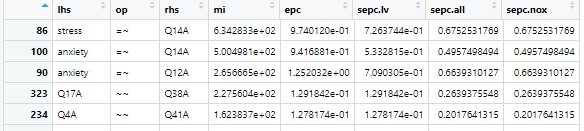
It looks like Q14A may load better on the stress factor. Since this aligns with theory, let’s make the change and see if the fit improves:
model.dass <-'
    stress =~ Q22A + Q6A + Q12A + Q39A + Q8A + Q14A + Q18A
    anxiety =~ Q2A + Q4A + Q41A + Q40A + Q28A + Q19A + Q20A
    depression =~ Q3A + Q42A + Q10A + Q26A + Q31A + Q17A + Q38A
    '
fit.dass <- cfa(model.dass, data = sample_df, missing = "fiml", estimator = "ML")
summary(fit.dass, fit.measures = TRUE, standardized = TRUE)

  Comparative Fit Index (CFI)                    0.952
  Tucker-Lewis Index (TLI)                       0.945


  RMSEA                                          0.053
  90 Percent confidence interval - lower         0.051
  90 Percent confidence interval - upper         0.055
  P-value RMSEA <= 0.05                          0.003


  SRMR                                           0.032
Again, we have some substantial fit improvement. If we still were not happy with our fit we could continue this process until we have a good fitting model, or further changes no longer make theoretical sense. Once we have established our model fits well, we use that model for our measurement invariance work.
Measurement Invariance
Just as in my previous post about measurement invariance (MI), we will attempt to achieve invariance based on individuals’ voting status (did, or did not, vote). We know from my previous post that we achieved strict invariance using this data and grouping variable. In that post I used change in CFI values > 0.01 to make the decision of whether or not to retain the more constrained model; however, for this example we will compare our models with an ANOVA test. Note that ANOVA does NOT function well when our sample is over a few hundred, so I would not normally use ANOVA to determine MI with this dataset. However we will use it here to demonstrate how to identify problem parameters when attempting to achieve MI. First, we need to run our configural model, which is just a multi-group CFA.
model.mi <- '
    stress =~ Q22A + Q6A + Q12A + Q39A + Q8A + Q14A + Q18A
    anxiety =~ Q2A + Q4A + Q41A + Q40A + Q28A + Q19A + Q20A
    depression =~ Q3A + Q42A + Q10A + Q26A + Q31A + Q17A + Q38A
'
fit.config <- cfa(model.mi, data = sample_df, missing = "fiml", group = "voted",  estimator = "ML")
summary(fit.config, fit.measures = TRUE, standardized = TRUE)
This code gives us a nicely fitting model, so we are free to move on to attempt weak invariance.
fit.weak <- cfa(model.mi, data = sample_df, missing = "fiml", group = "voted", group.equal = "loadings",  estimator = "ML")
summary(fit.weak, fit.measures = TRUE, standardized = TRUE)
anova(fit.config, fit.weak)

Chi-Squared Difference Test

            Df    AIC    BIC  Chisq Chisq diff Df diff Pr(>Chisq)
fit.config 372 259680 260539 2994.0
fit.weak   390 259704 260446 3054.1     60.146      18  1.938e-06 ***
---
Signif. codes:  0 ‘***’ 0.001 ‘**’ 0.01 ‘*’ 0.05 ‘.’ 0.1 ‘ ’ 1
The code above runs the weak invariance model by fixing all factor loadings to be equal between groups. Comparing the models using an ANOVA shows that we get a significant p-value, meaning the weak model fit the data significantly worse, which is NOT what we want. Measurement invariance is the assumption that a more constrained model fits the data equally well as a less constrained model (that you are measuring the same phenomenon in the same way across groups). So, what to do? Well, we can evaluate each of the parameters for their relative impact on model fit, and progressively free some parameters until we achieve a non-significant ANOVA.
We want to free parameters that have a statistically significant impact on model fit. Luckily lavaan has a couple of handy functions to help us out: lavTestScore and parTable. lavTestScore is a function that shows us each parameters’ contribution to model misfit. Ideally, we want to choose those parameters with small and significant p-values to free, thus making the largest improvement to our model fit. Let’s look at our weak model to see which parameters are giving us the most trouble.
df_weak_test <- lavTestScore(fit.weak)
df_weak_test <- (as_data_frame(df_weak_test[2]))
View(df_weak_test)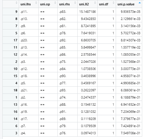
The table above is sorted so that the smallest p-values are on top. That is where we want to start freeing parameters. Normally you would free one parameter at a time and recheck the ANOVA p-value, stopping once we attain a non-significant p-value; however, in the interest of space, I will free the top four parameters all at once:
- p11 == p83
- p10 == p82
- p9 == p81
- p6 == p78
Unfortunately these parameter descriptions are not helpful for us to respecify our model, so we need parTable to gather more information. parTable shows the labels of all parameters in the model and lets us interpret the results from lavTestScore.
parTable(fit.weak)Here is a sample of what the parTable output looks like:

Using the table we can determine that:
- p11 == p83 is the loading of Q40A on anxiety
- p10 == p82 is the loading of Q41A on anxiety
- p9 == p81 is the loading of Q4A on anxiety
- p6 == p78 is the loading of Q14A on stress
So, lets free those loadings and rerun our weak MI model and ANOVA comparing the weak and configural models. We just need to add the “group.partial” argument to the cfa function to specify which parameters we want to free
fit.weak2 <- cfa(model.mi, data = sample_df, missing = "fiml", group = "voted", group.equal = "loadings", group.partial = c("anxiety =~ Q40A", "anxiety =~ Q41A", "anxiety =~ Q4A", "stress =~ Q14A"),  estimator = "ML")

summary(fit.weak2, fit.measures = TRUE, standardized = TRUE)

anova(fit.config, fit.weak2)

Chi-Squared Difference Test

            Df    AIC    BIC  Chisq Chisq diff Df diff Pr(>Chisq)
fit.config 372 259680 260539 2994.0
fit.weak2  386 259673 260441 3015.8     21.819      14    0.08242 .
---
Signif. codes:  0 ‘***’ 0.001 ‘**’ 0.01 ‘*’ 0.05 ‘.’ 0.1 ‘ ’ 1
Running the above code we can see that we now have a non-significant ANOVA p-value, meaning we have achieved partial weak invariance.
Now that we have achieved partial weak invariance we can test for strong invariance. To do so we carry over the model we used to achieve partial weak invariance.
fit.strong <- cfa(model.mi, data = sample_df, missing = "fiml", group = "voted", group.equal = c("loadings", "intercepts"), group.partial = "anxiety =~ Q40A",  estimator = "ML")

summary(fit.strong, fit.measures = TRUE, standardized = TRUE)

anova(fit.weak2, fit.strong)

Chi-Squared Difference Test

            Df    AIC    BIC  Chisq Chisq diff Df diff Pr(>Chisq)
fit.weak2  386 259673 260441 3015.8
fit.strong 404 259768 260419 3146.7     130.87      18  < 2.2e-16 ***
---
Signif. codes:  0 ‘***’ 0.001 ‘**’ 0.01 ‘*’ 0.05 ‘.’ 0.1 ‘ ’ 1
We can see that we once again have a significant anova test, meaning we need to further free some parameters. We can go through the same steps we did to achieve partial weak invariance to achieve partial strong invariance, although this time we will free intercepts, since that is what is constrained to be equal in the strong model. For example, we could add the top parameter contributing to the strong model misfit (Q14A) this way:
fit.strong <- cfa(model.mi, data = sample_df, missing = "fiml", group = "voted", group.equal = c("loadings", "intercepts"), group.partial = c("anxiety =~ Q40A", "anxiety =~ Q41A", "anxiety =~ Q4A", "stress =~ Q14A", "Q14A ~1),  estimator = "ML")

summary(fit.strong, fit.measures = TRUE, standardized = TRUE)
Similarly, once we achieve partial strong invariance we could investigate the parameters contributing to strict model misfit and sequentially free them in the same way demonstrated previously.
Establishing measurement invariance is an important part of creating valid survey instruments. Individuals interpret questions based on their experiences and backgrounds, meaning that two individuals might interpret questions quite differently. Measurement invariance is one statistical way we can help ensure that our surveys are valid for a range of diverse individuals.
***Check out the Github repository for this post to access the data and R script***
