Welcome to Part 2 of this three part series! If you have not read Part 1, and are unfamiliar with latent profile analysis, I recommend taking a few minutes to do that before you dive in here. Additionally, check out Spurk et al. (2020) for a succinct overview of the profile enumeration process. In this post we will use the National Financial Well-being survey dataset to construct a set of personal finance profiles. We will first model a number of profile solutions using different variance/covariance assumptions, then identify several candidate models to investigate in more detail, and finally select a single model to interpret and proceed with further analyses.
The first step in conducing a latent profile analysis is to mode the various possible variance/covariance structures. All profiles have freely estimated means, since means of the indicators variables are what make each profile unique. If means were equal between profiles they would all be the same. Since the purpose of LPA is to identify individuals who are different based on the selected indicator variables these profiles would be useless. There are six possible variance/covariance structures, and generally researchers choose to model between 2 – 10 profile solutions with each model type. For brevity’s sake, we will only use two model types and run 2 – 8 profile solutions with each model type. Oftentimes the final solution from an LPA analysis comes from one of the two bolded model types below so those are what we will use; however, in a real world application of LPA it is important to check solutions from each of the six model types.
- Varying means, equal variances, and covariances fixed to 0
- Varying means, equal variances, and equal covariances
- Varying means, varying variances, and covariances fixed to 0
- Varying means, varying variances, and equal covariances
- Varying means, equal variances, and varying covariances
- Varying means, varying variances, and varying covariances
Now that we have planned our analyses its time to decide how we want to conceptualize our personal finance profiles to select the indicator variables which we will use to construct our profiles. The National Financial Well-being survey is far-reaching and covers a wide range of knowledge and skills related to personal finance. Let’s say we are especially interested in financial well-being, financial skills, managing personal finances, and personal financial knowledge. Each of these constructs is measured by multiple survey items. Therefore, we can model our indicator variables in three ways: 1) as latent variables 2) as observed variables using composite means, or 3) as observed variables using factor scores. Ideally we would want to model latent constructs as latent variables, but in reality the complexity of LPA models often precludes using latent variables due to model convergence issues. Using factor scores is a nice middle ground, but in in our analysis here we will model our LPA indicators as composite means to keep things simple and focus on profile analysis and not measurement issues.
However, I did do some measurement work (CFAs and Cronbach’s alpha) to check the reliability of our personal finance variables and, for the most part, they were acceptable. The one exception was the three reverse coded items in the financial well-being scale. Those did NOT fit well, so I removed them for the remainder of the analyses. See the R script in the github repository linked at the end of this blog if you’re interested in checking that out.
Alright, let’s run some models using the tidyLPA R package!
profile_data <- select(fin_data, fin_wb, fin_sk, per_fin, fin_plan)
profile_data <- single_imputation(profile_data)

model1 <- estimate_profiles(profile_data,
                  n_profiles = 2:8,
                  variances = "equal",
                  covariances = "zero",
                  package = "mclust")

model2 <- estimate_profiles(profile_data,
                  n_profiles = 2:8,
                  variances = "equal",
                  covariances = "equal",
                  package = "mclust")
A few things to notice about the above code. First, we are using the “mclust” package to run these LPAs. The other option, if you have it installed, is to use Mplus. Mplus is nice because it is more flexible and you can save all of the Mplus output files to comb through the results in more detail. Also note that mclust can not handle any missing data in the indicator variables, so you need to use some sort of imputation method to estimate values for any missing data you might have. Luckily there are not many missing values in this data, so single imputation is a quick and reasonable choice. Finally we are estimating two model types using different variance/covariance structures and 2 to 8 profile solutions in each model type.
Awesome, we have our initial set of 14 models. Unfortunately, the easy part is over. Now we have to take our initial set of models and settle on a final solution. There are three main steps to selecting a final model:
- Use fit statistics to identify a subset of candidate models from the full original set.
- Consider theoretical interpretability and parsimony to select a final solution from the subset of models
- Check classification statistics to ensure the final model accurately classifies the observations
To identify a set of candidate models we can use a variety of fit statistics, but most commonly used are the BIC, AIC and BLRT. Lower values of BIC and AIC are better and we hope to see significant BLRT values (the BLRT compares the current profile solution to the previous one, with significant values indicating the current solution is a better fit). Note that you can compare fit statistics across model types (so a lower BIC is better, regardless of what model it is in). The code below demonstrates how we would go about evaluating possible solutions from model 1:
fit1 <- get_fit(model1)
get_estimates(model1)
get_data(model1)
The first function get_fit displays a variety fo fit statistics, get_estimates shows the means, variances, etc. of each profile in each class, and get_data will display individual class assignment and probabilities for each observation. Below are the fit statistics for each model type filtered for the most useful fit statistics using the compare_solutions function:
MODEL 1
compare_solutions(model1, statistics = c("BIC", "AIC", "BLRT_val", "BLRT_p"))
Model Classes    BIC       AIC      BLRT_val  BLRT_p
 1     2       58981.029  58893.109  5793.539  0.010
 1     3       57451.855  57330.119  1572.920  0.010
 1     4       56836.687  56681.136  657.453   0.010
 1     5       56721.440  56532.073  172.026   0.010
 1     6       56393.269  56170.086  363.609   0.010
 1     7       56083.938  55826.940  350.788   0.010
 1     8       55799.547  55508.733  327.447   0.010

MODEL 2
compare_solutions(model2, statistics = c("BIC", "AIC", "BLRT_val", "BLRT_p"))
 Model Classes BIC      AIC      BLRT_val     BLRT_p     Warnings
 3     2       55911.01 55782.51 875.09868171 0.00990099
 3     3       55319.67 55157.36 634.96134178 0.00990099
 3     4       55364.67 55168.54  -0.12766788 0.65346535 Warning
 3     5       55161.35 54931.40 257.62184410 0.00990099
 3     6       54802.82 54539.06 244.65688071 0.00990099 Warning
 3     7       54749.42 54451.84  -0.06214072 0.55445545 Warning
 3     8       54700.46 54369.07 335.61342687 0.00990099 Warning
Uh oh, looks like model 2 has some warnings. There are a number of reasons why this might be (model did not converge, logliklihood not replicated, small profile size, etc.), but generally this means we probably should not consider these solutions. Another method when evaluating models is to graph the BIC values. Normally, smaller BIC values indicate better model fit; however, sometimes the BIC just continues to decrease ad infinitum. In those cases we can look for an “elbow point”. The point at which the BIC starts to decline at a substantially lower rate than previously.
ggplot(fit2, aes(x = Classes, y = BIC)) +
    geom_line()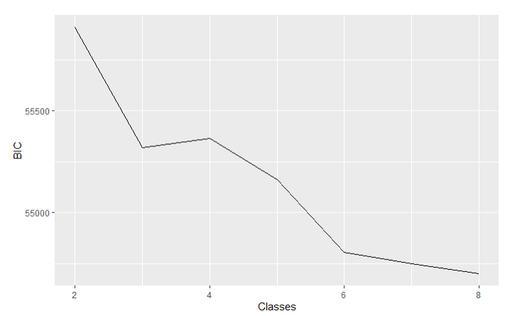
In the graph above the elbow point for model 2 appears to be at the three or six profile solution, but the six solution model is non-interpretable, so that can’t be our final solution.
Using our fit statistics table and graphs of BIC values we can conclude the ideal solution in either model is probably somewhere in the middle of the profile range. The BLRT is no help in model 1 since it is significant in all instances, but in model 2 it suggests either a three or six profile solution. Using the best available evidence from this step we will take a closer look at solutions with 3, 4, 5, and 6 profiles from model 1, and solutions with 3 and 5 profiles from model 2.
Now that we have a small subsample of candidate models we can consider theoretical and practical interpretability to help select a final solution. In this step we ask questions like: “Does this additional profile meaningfully add to my understanding of the phenomenon under study?”, “Do these combinations of indicators make theoretical sense?”, and “How many observations are in each profile?”. Graphing the means of these candidate models is a useful way to get a handle on things and help us understand what story the profile solutions are telling. Below are graphs from the two candidate solutions from model 2 (see this blog’s github repository for plot code). Note that the survey used a Likert-type scale for all items that ranged from 1 – 5 with 1 being the least desirable value and 5 being the most desirable value (scale labels were different depending on the construct).
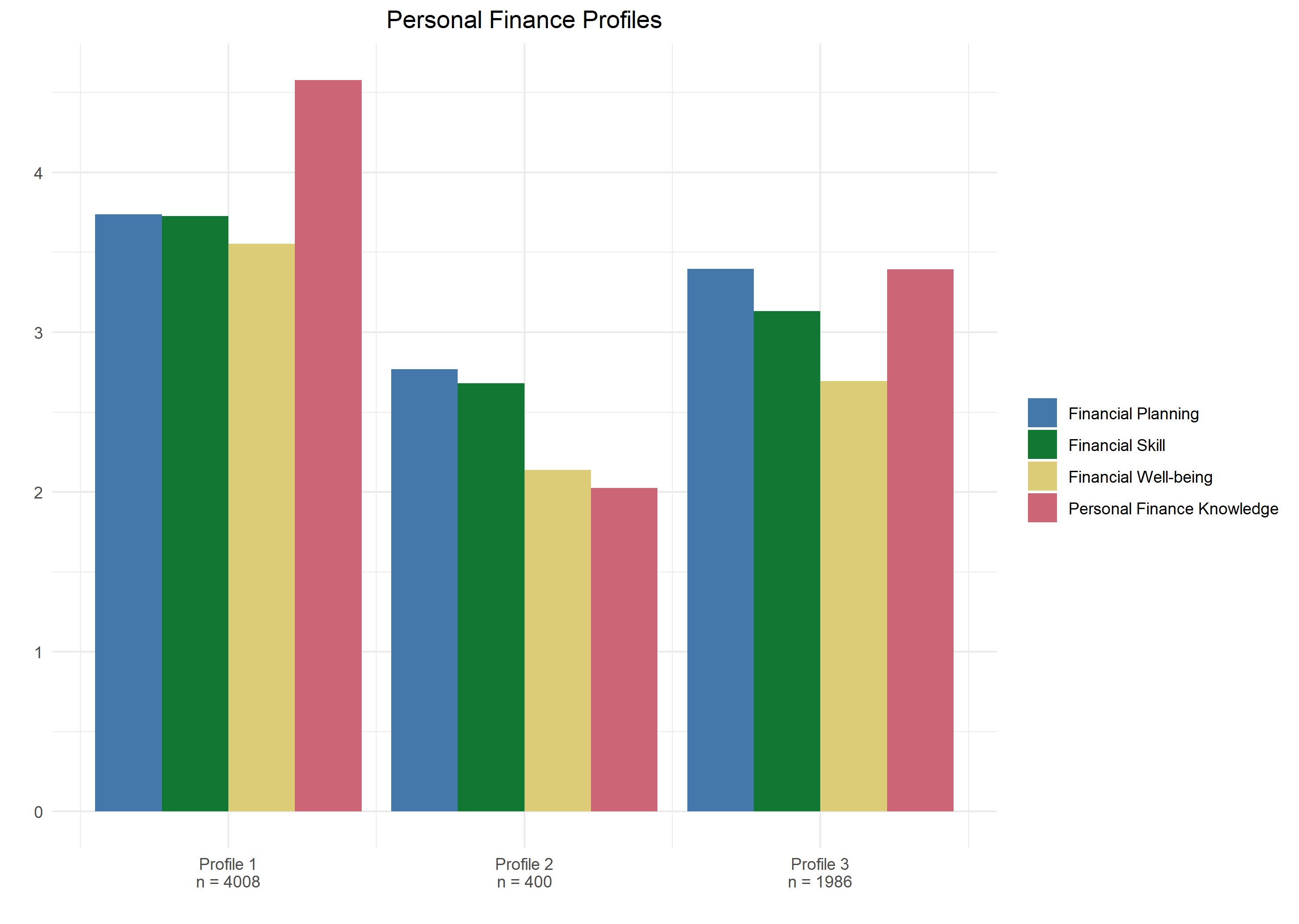
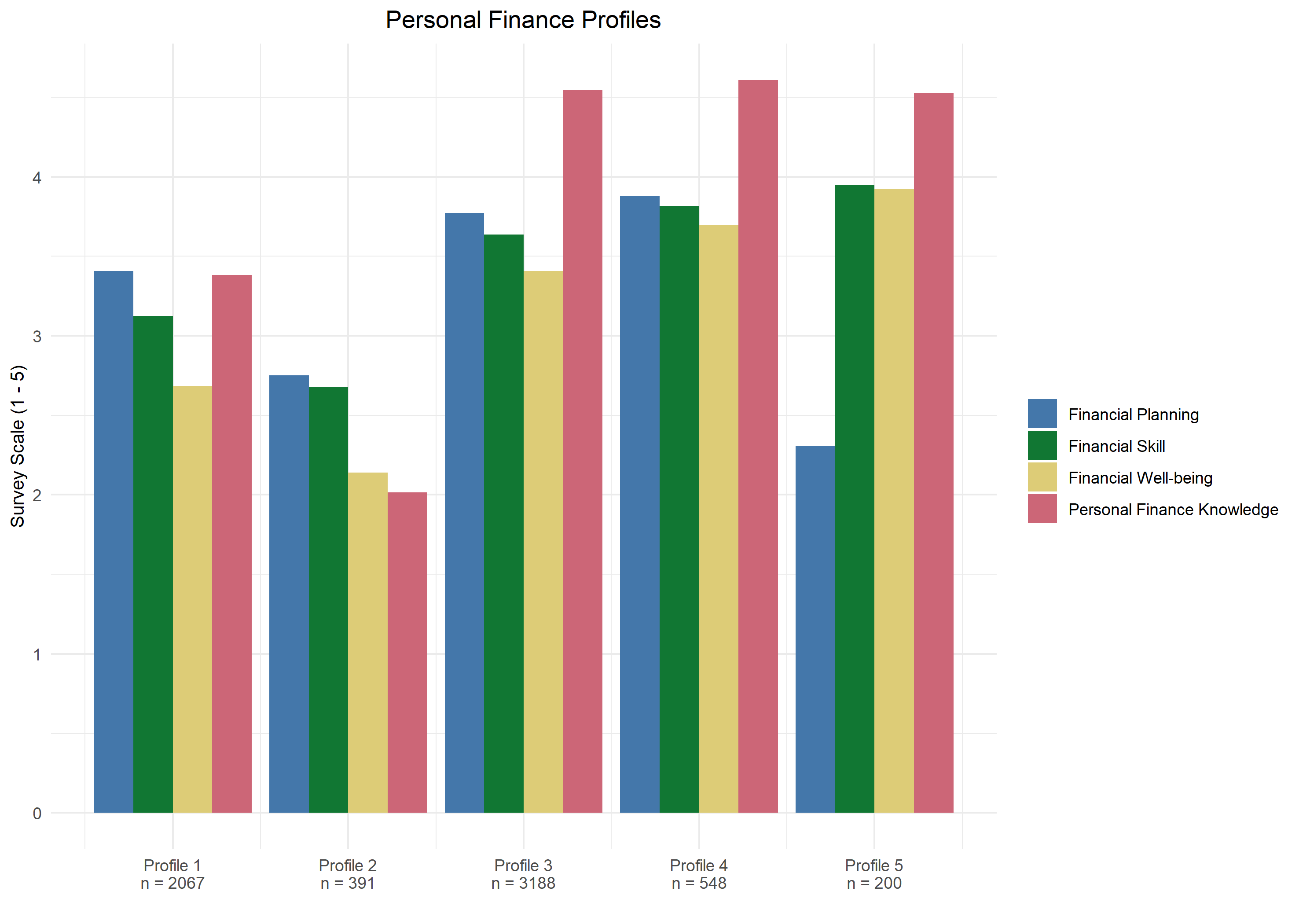
Wow! Graphs really help to better interpret the profiles and identify a final model that makes sense theoretically and practically. For example, profile 4 and profile 5 appear to describe meaningfully different populations of individuals. We can see that profile 4 has quite high means on all of the indicators, with an especially high personal finance knowledge mean. However, profile 5 has similar means on all indicators, except for financial planning which is substantially lower than the other three.
After considering the various candidate models we must settle on a final solution. Let’s say that after much consideration and hand wringing we select the model 2 five profile solution. There are a number of reasons to support our decision. As we previously discussed, the fit statistics suggest this model describes the data better than most other models. Second, the five profile solution in model 2 adds meaningful profiles compared to the three profile solution (e.g. profile 5 is not present in the three profile solution and describes a potentially important sector of the population). Third, the covariance structure of model 2 is more similar to the true relationship between the indicator variables. Correlations between indicators are all positive and moderate in size, suggesting some substantial covariance between them. Modeling the covariances as 0 (like in model 1) ignores this association. Lastly, the number of observation in each profile is acceptably large. A general rule of thumb is that at least 1% of the total observations should be in a profile to consider it valid. The smallest profile in this solution is 200 observations, or 3% of the total.
The final step is to confirm that our selected profile solution does an adequate job of categorizing observations into the correct profile using the entropy statistic. Generally we want to see entropy values above 0.7 and ideally above 0.8. Our solution only has a value of 0.6. Smaller values lower the confidence we have in the validity and reproducibility of our profiles. Its not a deal-breaker for model selection, but does suggest we need more evidence from multiple samples and studies before making strong conclusions.
One common question when interpreting LPA profiles is: “Which profiles are ACTUALLY different from one another?”. From the graph below we can see that profile 3 and profile 4 from the five profile solution look quite similar, so are those two profiles statistically different from one another?

One way to find out is by using a MANOVA with some post-hoc tests.
#Preparing dataset
m2_data <- get_data(model2)
man_df <- filter(m2_data, classes_number == 5 & Class_prob == 1)
man_df$Class <- as.factor(man_df$Class)

#Running MANOVA and ANOVA models and checking for overall model significance.
model.man <- manova(cbind(fin_wb, fin_sk, fin_plan, per_fin) ~ Class, data = man_df)
summary(model.man, test = "Wilks")
summary.aov(model.man)

#Pairwise comparisons between all profiles using the financial well-being indicator.
model.fin_wb <- aov(man_df$fin_wb ~ Class, data = man_df)
summary(model.fin_wb)
tukey.fin_wb <- TukeyHSD(model.fin_wb)
tukey.fin_wb

$Class
        diff        lwr       upr     p adj
2-1 -0.5266797 -0.6424039 -0.4109556     0
3-1  0.6417896  0.5825314  0.7010478     0
4-1  2.1124560  2.0116313  2.2132807     0
5-1  1.3567260  1.2013328  1.5121193     0
3-2  1.1684694  1.0560283  1.2809104     0
4-2  2.6391358  2.5002219  2.7780497     0
5-2  1.8834058  1.7009818  2.0658298     0
4-3  1.4706664  1.3736276  1.5677052     0
5-3  0.7149364  0.5619724  0.8679004     0
5-4 -0.7557300 -0.9290853 -0.5823747     0
The above code demonstrates the process of using a MANOVA and ANOVA to check for overall model significance and one set of pairwise comparisons between profiles on the financial well-being indicator. We could finish off this analysis by copying and slightly modifying the last chunk of code and using it to compare profiles on the remaining personal finance indicators. Notice that all profiles are significantly different from one another on the financial well-being indicator. As it turns out there is only one non-significant result in the entire sample of pairwise comparisons, that on personal finance knowledge between profile 3 and profile 5. This is great news! It means that individuals in separate profiles truly do experience personal finance differently.
Now we are ready to interpret our final solution! This is the part of the analysis where you get to use your domain knowledge to add some context to the profiles. A couple things jump out immediately as I look at the graph of our final solution (five profiles). First, as we saw earlier, is that individuals in profile 5 rate their financial planning abilities substantially lower than the other measures of personal finance. This suggests that there is a subset of people who are quite knowledgeable and skilled in the realm of personal finance, but do not make plans regarding their financial life. Perhaps they are comfortable enough in their financial situation that they feel no need to plan? Additionally, in profile 2 the personal finance knowledge indicator is substantially below the means of financial well-being and financial skill. This suggests that even though this population of individuals perceives their well-being and skill to be moderately high, they still perceive their knowledge about finances to be moderately low. This is an interesting set of people. Perhaps they know how to navigate finances at a high level, but pay a financial adviser to take care of the details? We might have to go back and evaluate the actual survey questions to help us explain this profile.
That about wraps up this whirlwind tour of latent profile analysis. Notably, it can be quite time consuming to run all 6 model types, with with many profile solutions. LPA is computationally expensive, so depending on your computer’s processing ability just running all the models can take a few hours. Then you need to organize the fit statistics, graph several potential solutions, run the MANOVA, interpret your profiles, name them, etc. etc. All in all, count on the entire process taking more than a couple of days. That being said, the results are a unique and impactful way to describe how a set of meaningfully related constructs vary simultaneously. Additionally, these profiles can then be predicted by, or predict, other variables of interest. In Part 3 of this series we do just that!
***Check out the github repository associated with this post to access the data and Rscript***
References
Spurk, D., Hirschi, A., Wang, M., Valero, D., & Kauffeld, S. (2020). Latent profile analysis: A review and “how to” guide of its application within vocational behavior research. Journal of Vocational Behavior, 120, 103445. https://doi.org/10.1016/j.jvb.2020.103445
