There are a few industries that seem to perennially have the reputation of terrible customer service: internet providers, phone companies…and airlines.
How often have you head someone gush about the amazing customer care and support they received from an airline, or raved about how enjoyable their flight was (especially if not business or first class)? Probably not a whole lot, especially in comparison to how many horrors stories you have seen and heard about flights. When I fly I’m happy to walk away from the experience thinking, “Well, that wasn’t terrible.”
Some of the blame probably lies on profit maximization by the airline companies, but flying is also just a difficult and expensive thing to do safely and reliably. Airlines are expected to send somewhere around 6 million people every day hurtling through the sky at over 500 miles per hour and get them to their destination smoothly and on time. Pretty amazing when you think about it. Nevertheless, pleased customers are repeat customers, so airlines are interested in how satisfied patrons are with their flight experience to adapt and improve processes and services to gain an ever larger slice of market share.
To explore how satisfied customers are with a flight experience we will use the Invistico Airlines Customer Satisfaction survey. This real-world (anonymized) survey based dataset features 23 variables and over 120,000 responses examining various factors that theoretically impact whether customers feel satisfied or dissatisfied with a flying experience on Invisitco Airlines. Let’s go ahead, load the data, and check it out.
library(tidyverse)
library(psych)
library(car)
library(reshape2)
library(ggplot2)
library(cowplot)

airline <- read_csv("yourfilepathhere.csv")
Since we are interested in learning whether customers were satisfied (or not) with their flying experience, a logistic regression is a useful analytical method to use. Logistic regression allows us to predict the likelihood of a categorical outcome using any number of categorial or continuous variables. Conveniently, our dataset has a nice categorical variable which indicates if customers were satisfied or dissatisfied with a recent flying experience.
Data Cleaning and Pre-Model Set-Up
This dataset is mostly clean and ready to go, but there are still a few quality of life changes that make the data easier to work with (e.g. changing character vectors to numeric or factor variables, renaming variables, etc.). We also need to replace “0” values in this dataset with NAs.
#Renaming variables with spaces to make them easier to work with
airline <- rename(airline, inflight_entertainment = "Inflight entertainment", onboard_service = "On-board service", leg_room = "Leg room service", online_booking = "Ease of Online booking", online_boarding = "Online boarding", online_support = "Online support", food_drink = "Food and drink")

#Recoding some character vectors into numbers or factors
airline$satisfied <- (car::recode(airline$satisfaction, c("'satisfied' = 1; 'dissatisfied' = 0")))
airline$female <- car::recode(airline$Gender, c("'Female' = 1; 'Male' = 0"))
airline$economy <- car::recode(airline$Class, c("'Eco' = 1; 'Business' = 0"))
airline$economy <- as.numeric(airline$economy)

#Replacing 0 with NA for survey questions (likert scale is 1-5 in this survey, so we are assuming 0 means a skipped question)
airline2 <- select(airline, food_drink:online_boarding)
airline <- select(airline, !(food_drink:online_boarding))

airline2 <- na_if(airline2, 0)
airline <-cbind(airline, airline2)
Is it hot in here? Oh wait…that’s just a correlation heatmap.
Great! Our dataset is looking good now. Next, we need to decide which variables to include in our analysis. There are a few ways to go about this. First, we should always include variables we are interested in. This could be based on theory, what is important to stakeholders, or based on some quantitative method. For this post we will use a correlational heatmap to identify which variables have some substantial covariance with our outcome of interest (customer satisfaction), and are thus likely to be significant predictors.
cordat <- select_if(airline, is.numeric)

cormat <- round(cor(cordat, use = "pairwise.complete.obs"), 2)

melted_cormat <- melt(cormat)
head(melted_cormat)

dist <- as.dist((1-cormat)/2)

hc <- hclust(dist)
cormat <- cormat[hc$order, hc$order]

melted_cormat <- melt(cormat)

ggplot(data = melted_cormat, aes(x = Var1, y = Var2, fill = value)) +
  geom_tile() +
  geom_text(aes(Var2, Var1, label = value), color = "black", size = 4) +
  theme(axis.text.x = element_text(angle = 45, vjust = 1.05, hjust = 1.2)) +
  scale_fill_gradient2(mid="#FBFEF9",low="#0C6291",high="#A63446",  limits=c(-1,1)) +
  labs(y = "", x = "")
After running the above code we get the following heatmap:
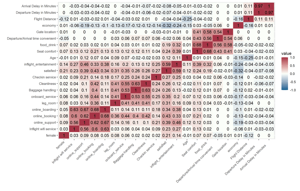
There is no hard and fast rule as a correlation cutoff when selecting variables from a heatmap. To keep things manageable, we will use a cutoff of >0.3 for inclusion in the logistic regression model. This means we will include a total of 8 predictor variables ( 7 indicated from the correlation heatmap and a gender variable because stakeholders may be interested in it).
Modeling Customer Satisfaction with a Logistic Regression
The time as come to run our logistic regression model!
fit <-glm(satisfied ~ female + economy + inflight_entertainment + onboard_service + leg_room + online_boarding + online_booking + online_support, data = airline, family = "binomial")
summary(fit)

Coefficients:
                        Estimate Std. Error  z value Pr(>|z|)
(Intercept)            -7.717212   0.051722 -149.204  < 2e-16 ***
female                  0.854042   0.017136   49.839  < 2e-16 ***
economy                -1.159688   0.017246  -67.246  < 2e-16 ***
inflight_entertainment  1.135288   0.008723  130.152  < 2e-16 ***
onboard_service         0.362962   0.007954   45.633  < 2e-16 ***
leg_room                0.319963   0.007481   42.769  < 2e-16 ***
online_boarding         0.051773   0.009758    5.306 1.12e-07 ***
online_booking          0.405705   0.010249   39.583  < 2e-16 ***
online_support          0.071152   0.009217    7.720 1.16e-14 ***
---
Signif. codes:  0 ‘***’ 0.001 ‘**’ 0.01 ‘*’ 0.05 ‘.’ 0.1 ‘ ’ 1
At the top of the code chunk above we see our logistic regression model, then the results of the model after running the summary() function. Good news! All of the predictors we included have a significant impact on customer satisfaction. Before we celebrate too much, let’s make sure our overall model fits well.
Enter McFadden’s (1974) pseudo R squared. Generally, pseudo R squared values between 0.2 and 0.4 signify excellent model fit (meaning the model fits substantially better than the null model – one with no predictors). Running the code below we get an pseudo R squared value of 0.45, so our model fits well.
ll.null <- fit$null.deviance/-2
ll.fit.model <- fit$deviance/-2

1 - ll.fit.model / ll.null

1 - pchisq(2*(ll.fit.model - ll.null), df = (length(fit$coefficients)-1))
Now, let’s convert our coefficients to odds ratios and pull out point estimates and confidence intervals. Logistic regression coefficients are given in logits (log of the odds). Logits are notoriously difficult to make sense of, odds ratios are much more interpretable.
exp(coef(fit))
exp(confint(fit))
round(cbind(ORs = exp(coef(fit)), exp(confint(fit))), digits = 3)

                       ORs   2.5 %  97.5 %
(Intercept)            0.000 0.000  0.000
female                 2.349 2.272  2.429
economy                0.314 0.303  0.324
inflight_entertainment 3.112 3.059  3.166
onboard_service        1.438 1.415  1.460
leg_room               1.377 1.357  1.397
online_boarding        1.053 1.033  1.073
online_booking         1.500 1.471  1.531
online_support         1.074 1.055  1.093
Finally, we can now interpret our results to see what we can learn about airline customer satisfaction! Logistic regression results and odds ratios are notoriously difficult to interpret, so here we go.
Results – Interpreting Odds Ratios
Let’s interpret our coefficients (now in odds ratios instead of logits). Odds ratios equal to 1 indicate the predictor has no impact on the outcome. Odds ratios of less than one indicate a lower likelihood of the outcome, and odds ratios greater than 1 indicate a higher likelihood of the outcome.
Looking at the “female” variable we see it has an odds ratio of 2.35. We can interpret this as: The odds of that a female will be satisfied with a flight are 2.35 times higher than males. Note that we are using odds here, not probability. Saying the ODDS of a satisfied customer is 2.35 times higher is not the same as saying the probability is 2.35 times higher. Close, but not equal.
Now let’s look at a continuous variable, leg room (coefficient = 1.377). The leg room variable is a survey question asking customers to rate their satisfaction with the amount of leg room they had from 1 (not satisfied) to 5 (very satisfied). We can say that: For every 1 point increase in leg room the odds of an individual being satisfied increases by 35%. Not bad! Maybe airlines should take a look at this analysis when designing airplane interiors…
Finally, let’s take a look at the economy variable. This variable is coded as a customer who booked an economy ticket (coded as 1), or a business/1st class ticket (coded as 0). The coefficient for the economy variable is below 1 (0.314). Odds ratios of less than 1 mean there is a lower likelihood of the the outcome (in our case, being satisfied with the flight). So we can say: The odds of being satisfied when flying economy is almost 70% lower compared with flying business or first class. The real question is…does the free champagne up front explain that difference, or is it the hot towels?
Graphing Predicted Probabilities to Check the Usefulness of our Model
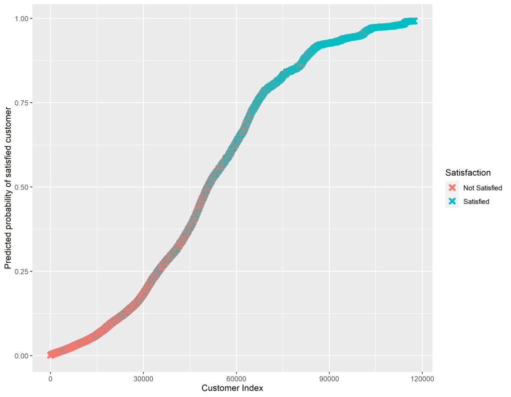
A final, useful step, is graphing the predicted probabilities for each individual in our dataset to broadly see how well our logistic regression has done at modeling the data.
We expect that if our model predicts a high probability that a customer is satisfied, then that customer should actually be satisfied in the dataset. A predicted probabilities graph plots each customer against their probability of being satisfied. Since the satisfaction variable is a factor we can easily tell R to differentiate by color those customers who were coded as satisfied in the dataset and those who were not satisfied.
#Since glm() uses listwise deletion we need to filter out observations with NA values on any predictor from our original dataset in order for the number of observations to match the output from our model.
airline_pp <- filter(airline, !is.na(economy)) %>%
                   filter(!is.na(inflight_entertainment)) %>%
                   filter(!is.na(onboard_service)) %>%
                   filter(!is.na(leg_room)) %>%
                   filter(!is.na(online_boarding)) %>%
                   filter(!is.na(online_booking)) %>%
                   filter(!is.na(online_support))

#Making a new data frame that matches the predicted outcome with the actual outcome, and ranks them.
predicted_data <- data.frame(probability.of.satisfied = fit$fitted.values, satisfied = airline_pp$satisfied)
predicted_data <- predicted_data[
  + order(predicted_data$probability.of.satisfied, decreasing = FALSE),]
predicted_data$rank <- 1:nrow(predicted_data)

#Graphing the new data.
predicted_data$satisfied <- as.factor(predicted_data$satisfied)
levels(predicted_data$satisfied) <- c("Not Satisfied", "Satisfied")

ggplot(data = predicted_data, aes(x = rank, y = probability.of.satisfied)) +
  geom_point(aes(color = satisfied), alpha = 1, shape = 4, stroke = 2) +
  labs(x = "Customer Index", y = "Predicted probability of satisfied customer",     color = "Satisfaction")

ggsave("predicted_probs.png", width = 9)
The code above gives us the graph below. We can see that those customers who were coded as “Not Satisfied” in the dataset had a low predicted probability of being a satisfied customer from our model. Similarly, our model predicted a high probability of satisfaction for those customers who were coded as “Satisfied” in the dataset.
That wraps up our exploration of airline customer satisfaction. Hopefully a major airline executive will read this post, make all seats first-class, provide us with free wifi, and ensure we have copious amounts of legroom!
*** Check out the Github repository associated with this post to access the data and R script***
References
McFadden, D. (1974) “Conditional logit analysis of qualitative choice behavior.” Pp. 105-142 in P. Zarembka (ed.), Frontiers in Econometrics. Academic Press. http://eml.berkeley.edu/~mcfadden/travel.html
